Theme Comparison

Overview

The package provides two ggplot2 themes:

• theme_t2m(): Clean, minimal theme with white background and viridis palette
• theme_solaris(): Warmer aesthetic with cream background and gold/amber palette

Both themes automatically detect and style ggraph network plots.

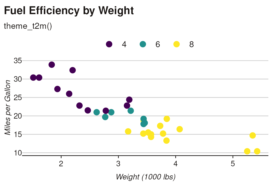
Theme Text2map

The default theme optimized for standard visualizations:

ggplot(mtcars, aes(wt, mpg, color = factor(cyl))) +
  geom_point(size = 4) +
  scale_color_viridis_d() +
  theme_t2m() +
  labs(
    title = "Fuel Efficiency by Weight",
    subtitle = "theme_t2m()",
    x = "Weight (1000 lbs)",
    y = "Miles per Gallon",
    color = "Cylinders"
  )

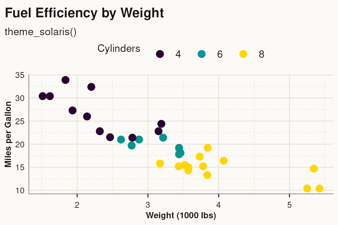
Theme Solaris

A warmer theme with cream background:

ggplot(mtcars, aes(wt, mpg, color = factor(cyl))) +
  geom_point(size = 4) +
  scale_color_solaris_d() +
  theme_solaris() +
  labs(
    title = "Fuel Efficiency by Weight",
    subtitle = "theme_solaris()",
    x = "Weight (1000 lbs)",
    y = "Miles per Gallon",
    color = "Cylinders"
  )

Side-by-Side Comparison

Compare both themes with identical data:

p1 <- ggplot(mtcars, aes(wt, mpg, color = factor(cyl))) +
  geom_point(size = 3) +
  scale_color_viridis_d() +
  theme_t2m() +
  labs(title = "theme_t2m()", color = "Cylinders") +
  theme(legend.position = "none")

p2 <- ggplot(mtcars, aes(wt, mpg, color = factor(cyl))) +
  geom_point(size = 3) +
  scale_color_solaris_d() +
  theme_solaris() +
  labs(title = "theme_solaris()", color = "Cylinders") +
  theme(legend.position = "none")

p1 | p2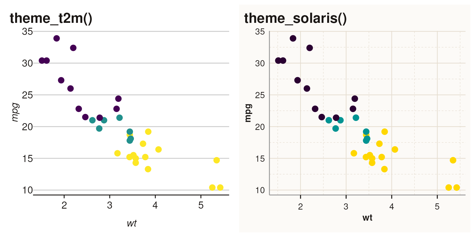

Faceted Plots

Both themes support faceted visualizations. The strip styling differs between themes:

p1 <- ggplot(mtcars, aes(wt, mpg)) +
  geom_point(size = 3) +
  facet_wrap(~cyl) +
  scale_color_viridis_d() +
  theme_t2m() +
  labs(title = "theme_t2m()", color = "Cylinders") +
  theme(legend.position = "none")

p2 <- ggplot(mtcars, aes(wt, mpg)) +
  geom_point(size = 3) +
  facet_wrap(~cyl) +
  scale_color_solaris_d() +
  theme_solaris() +
  labs(title = "theme_solaris()", color = "Cylinders") +
  theme(legend.position = "none")

p1 | p2
#> Ignoring unknown labels:
#> • colour : "Cylinders"
#> Ignoring unknown labels:
#> • colour : "Cylinders"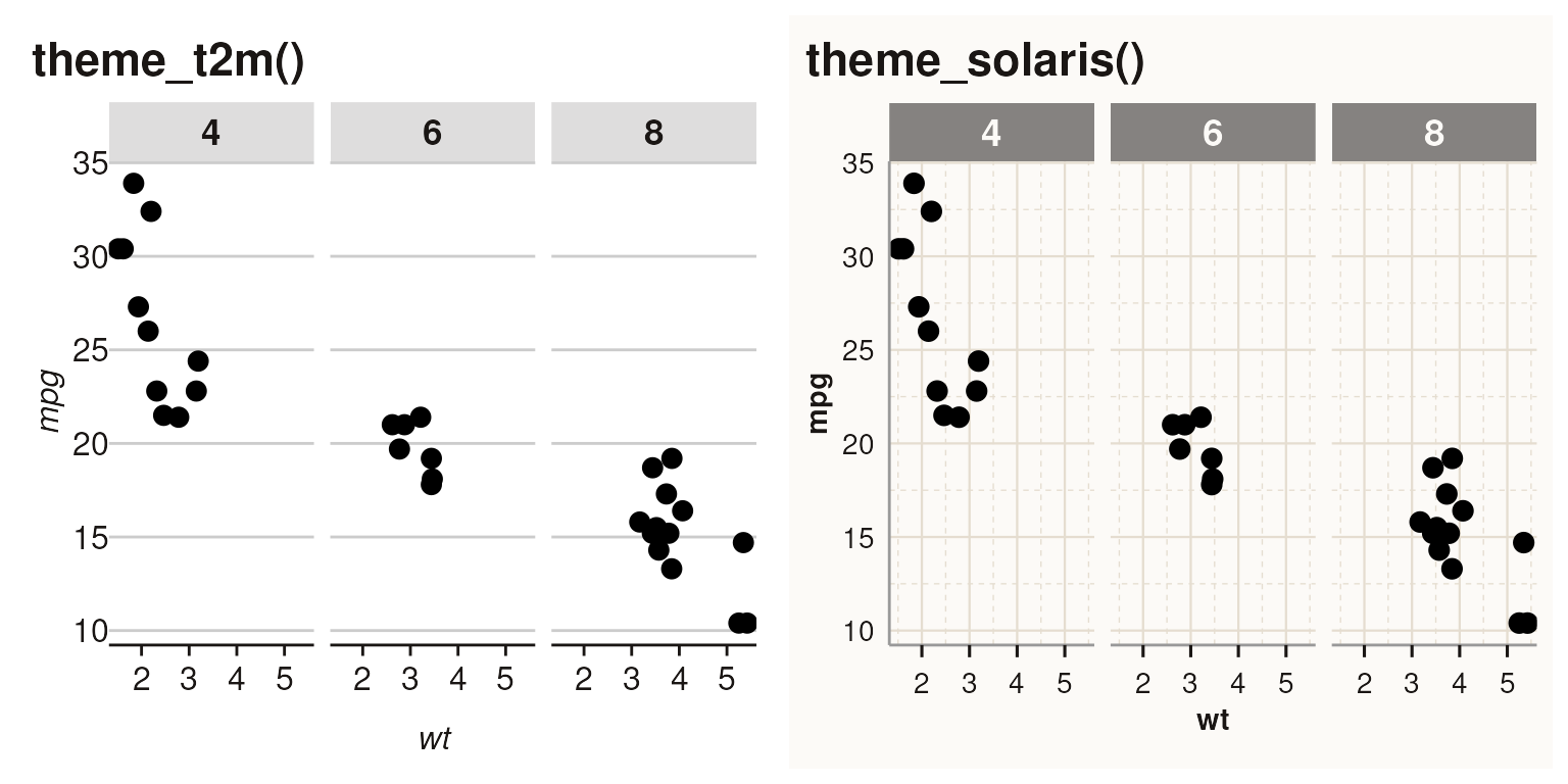

Key differences in facet strips: - t2m: Light gray background (#dedddd) with black bold text - solaris: Warm gray background (#858280) with cream text

Print vs Screen Medium

Both themes support a medium parameter for print optimization:

• medium = "screen" (default): Optimized for digital displays
• medium = "print": Darker colors, heavier lines for better physical reproduction

# Screen medium (default)
p_screen <- ggplot(mtcars, aes(wt, mpg, color = factor(cyl))) +
  geom_point(size = 3) +
  scale_color_solaris_d() +
  theme_solaris(medium = "screen") +
  labs(title = "medium = 'screen'", color = "Cylinders") +
  theme(legend.position = "none")

# Print medium
p_print <- ggplot(mtcars, aes(wt, mpg, color = factor(cyl))) +
  geom_point(size = 3) +
  scale_color_solaris_d() +
  theme_solaris(medium = "print") +
  labs(title = "medium = 'print'", color = "Cylinders") +
  theme(legend.position = "none")

p_screen | p_print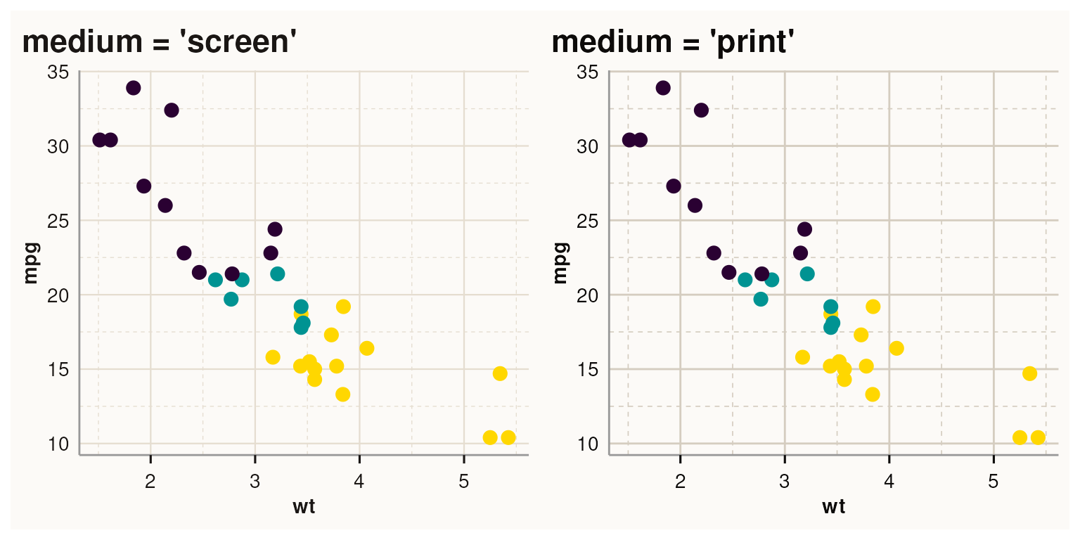

Print medium adjustments: - Darker text: #0d0b0a vs #1a1614 - Darker grid lines: +0.1 linewidth - Darker grid colors: #d5cdc0 (solaris), #aaaaaa (text2map)

When to Use Which Theme

Scenario	Recommended Theme
Academic papers, white background	theme_t2m()
Warm presentations, printed materials	theme_solaris()
Dark background slides	theme_t2m() + inferno palette
Colorblind accessibility	viridis palette (either theme)
Grayscale printing	theme_t2m() + grayscale palette

Using with set_theme()

The set_theme() function configures both the theme and palette globally:

# Set text2map theme with viridis (default)
set_theme()

# Set solaris theme
set_theme(palette = "solaris")

# Set print medium
set_theme(medium = "print")

# Combine options
set_theme(palette = "solaris", medium = "print")

For patchwork plots, use explicit scale functions instead of set_theme() to avoid lazy evaluation issues:

p1 <- ggplot(mtcars, aes(wt, mpg, fill = factor(cyl))) +
  geom_bar(stat = "identity") +
  scale_fill_viridis_d() +
  theme_t2m() +
  labs(title = "theme_t2m() + viridis") +
  theme(legend.position = "none")

p2 <- ggplot(mtcars, aes(wt, mpg, fill = factor(cyl))) +
  geom_bar(stat = "identity") +
  scale_fill_solaris_d() +
  theme_solaris() +
  labs(title = "theme_solaris() + solaris") +
  theme(legend.position = "none")

p1 | p2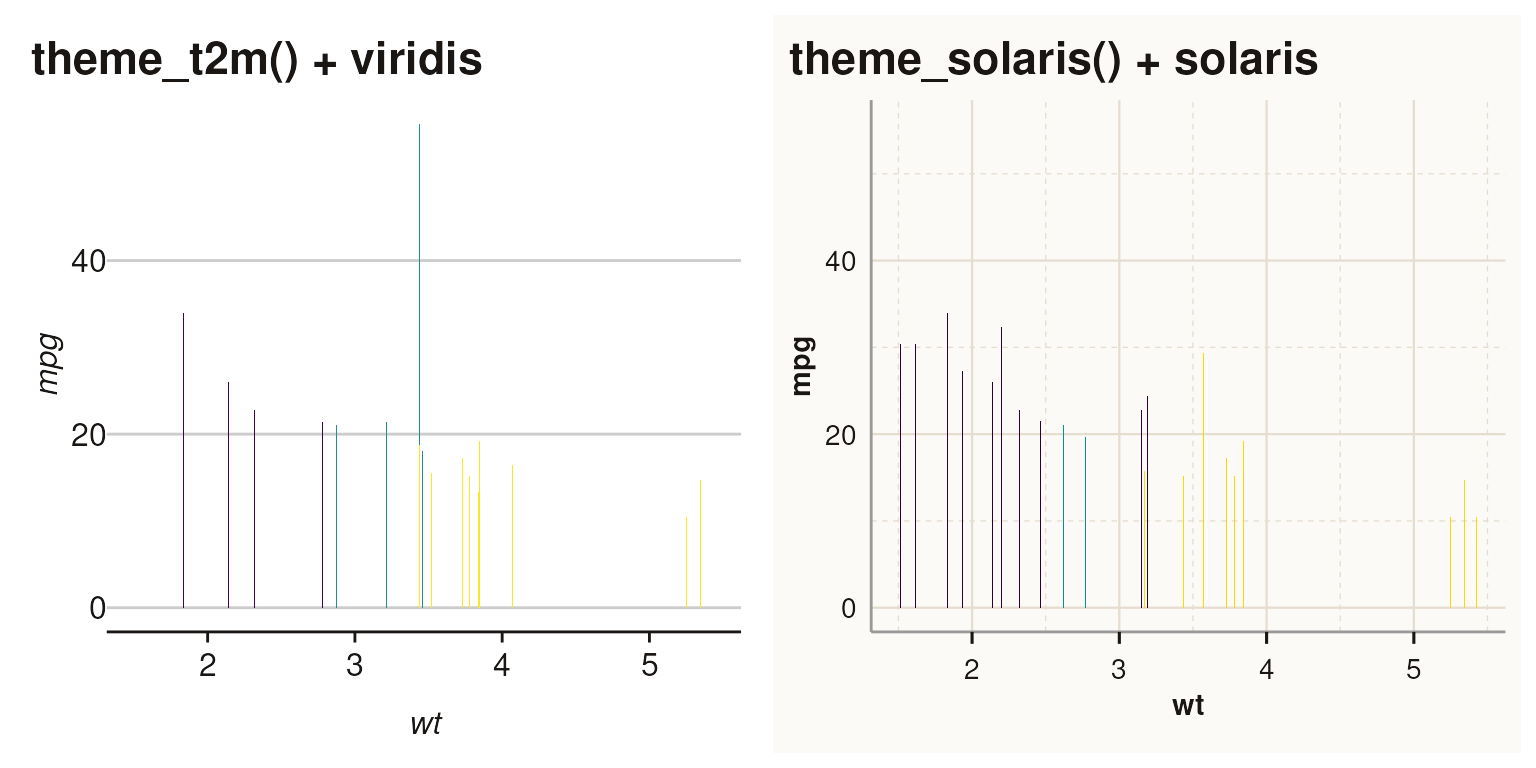

See vignette("color_palettes", package = "text2map.theme") for detailed palette comparisons.