Recover Human Knowledge from Word Embeddings
Dustin S. Stoltz
2026-07-19
Source:vignettes/articles/recover-human-knowledge-from-word-embeddings.Rmd
recover-human-knowledge-from-word-embeddings.RmdWord Embeddings and Human Knowledge
In a recently published study (Grand et al. 2022) on “semantic projection” (see here for an unpaywalled preprint), the authors “recover” human knowledge from word embeddings. This technique is increasingly common in word embeddings research because it can be used for such a variety of properties. For example, judging the relative size or dangerousness of an object, or even how “graspable” an object is (Fulda et al. 2017). This is, in essence, Osgood’s classic “semantic differentials,” but instead of asking people to rank objects along various scales, we can induce these rankings from how people use words.
What is really exciting about this line of research is that embeddings are only picking up on the information provided by word co-occurrence, which has (potentially) important implications for how we, humans, learn and reason (see Arseniev-Koehler 2021; Arseniev-Koehler and Foster 2020; Bender and Koller 2020).
Rather than dive into the theoretical side, let’s just demonstrate
how to perform the task using R. A few points to keep in
mind. Word embeddings summarize a word’s contexts across of a variety of
unique instances. When we engage in “semantic projection” we are
post-processing or fine-tuning the embeddings in an attempt to
re-specify the context.
Performing Semantic Projection with Word Embeddings
Projection
Let’s say we have a two-dimensional space. Any point in that space can be defined or located using two numbers, one for each dimension. Now, let’s say we want to “reduce” the dimensions of that space from two to just one. We will lose some information, but sometimes summarizing is useful.
We can move from two-dimension to one-dimension using projection. It’s not unlike shining a light in front of an object and casting it’s shadow onto a wall. The object’s position is now “projected” on to a flat plane.
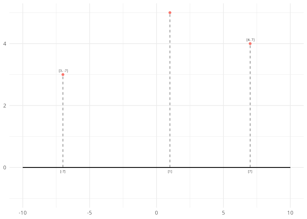
In the figure, two dimensional points are reduce to a position along a single dimension (here the X-axis). At least as it relates to this single dimension, we can now compare each points’ relative position. Where things become tricky is that the math will allow us to move well beyond the one- two- or three-dimensional space that we find intuitive. Walking through an actual example with word embeddings can help.
Get Pre-Trained Embeddings
The authors (Grand et al. 2022) use the
pretrained GloVe
Embeddings – although they also tested it on fastText, word2vec,
ELMo and BERT. Here, we will use the pretrained fastText Embeddings. We can download
them directly from the fastText website into our R session like so (you
can also checkout fasttextM
from which this code was borrowed):
ft_url <- paste0("http://dl.fbaipublicfiles.com/",
                 "fasttext/vectors-wiki/wiki.en.vec")
h <- new_handle()
handle_setopt(h, range = "0-1200000000")
res <- curl_fetch_memory(ft_url, h)

ft_wv <- mstrsplit(res$content,
                sep = " ", nsep = " ",
                type = "numeric",
                skip = 1L, ncol = 300L)
This will take a minute to download, and should be around 460,000 rows and 300 columns (if you increase the “range,” you will download vectors for more words). This means we have word vectors for the four hundred and sixty thousand most common words in the original training corpus, and our vectors are 300 dimensions long.
Semantic Projections
We can take this basic idea of casting the shadow of an object onto a
surface and instead “project” each of our word embeddings onto a line.
How do we define this line? We construct what we call a semantic
direction (Taylor and Stoltz
2021), or a vector that points toward some location in the
embedding space and away from another location. The most well-known
example of this is defining a direction from masculine to feminine (and
vice versa), and using it to measure the gender bias of a given word,
such as an occupational title. But, we can use this technique for all
sorts of things. text2map has a general function for
creating semantic directions (and using a few different methods), but
here is the basic pieces:
anchor_1 <- ft_wv["huge", , drop = FALSE]
anchor_2 <- ft_wv["tiny", , drop = FALSE]

sem_dir <- anchor_1 - anchor_2
That’s it! Take the vector for one “anchor” term and subtract it from
the other. This direction will point toward “huge,” but we
could also go the opposite direction by just swapping the order. The
other consideration is that words can have multiple senses. By using a
few anchor terms, we can try to be more precise about our intended
meaning. We make all this easy with get_direction().
# create anchor list
size <- data.frame(
  add = c("huge", "big", "large", "enormous"),
  subtract = c("tiny", "small", "little", "microscopic")
)

sem_dir <- get_direction(anchors = size, wv = ft_wv)
You’ll notice the output is just a vector in the same dimensions as our word embeddings (here 300). This is, in a sense, a “pseudo-word” vector, induced from the space itself.
Cosine Similarity
As our new vector is in the same “space” as the original word embeddings, we can compare the original word vectors directly with this new semantic direction vector. Let’s pick a few animals and put them in a “dictionary” (note that they must also be in the embeddings).
dict <- c("mouse", "dog","cat",
          "elephant", "cow", "pig",
          "grizzly", "horse")
We can measure how “close” a word’s vector is from the “huge” side of our semantic direction (and thus distance from “tiny”) in the same way we can measure gender bias by it’s “distance” from the gender direction. Typically, we do this by using cosine similarity. Cosine measures the angle between two points. An angle of zero would mean the vector is precisely the same as one side of our direction. So that larger numbers translate to greater similarity, though, we will use the inverse called cosine similarity. Here a 1 would mean the vector is precisely the same as one side of our direction, while a -1 would mean it is precisely the opposite, with a zero indicating the vector leans toward neither side.
We’ll use the function from text2vec. Since the output
will be a list of similarities, we will also reshape it into a
data.frame.
sims <- sim2(sem_dir, ft_wv[dict, ], method = "cosine")

df_sims <- data.frame(direction = sims[1, ],
                      term = colnames(sims))
Visualize Semantic Similarities
Using fct_reorder(), we will order our words by how
“close” they are to the “huge” side of our semantic direction, and then
pipe it to ggplot() to create a simple bar chart.
coord_flip() tips the plot over so it’s easier to read.
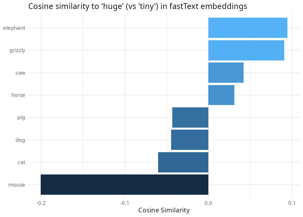
Importantly, this is not a measure of objective size, but something akin to a summary of the subjective understanding of relative size based on how a language community happens to use the words for these animals. Specifically, “meaning” is being equated to the lexical contexts in which the terms for these animals tends to be used.
Visualizing Semantic Projection
But wait, what about the nice three-dimensional plot from Grand et al. (2022)? Cosine similarity converts distances to a single number (i.e. a scalar). Instead, we could keep the coordinates of the projection on to the line. In the original example, we projected our points onto the X-axis. The actual projected coordinates for the point that was [4, 7] became [0, 7] if we were to retain our two-dimensional space.
When we use semantic projection with word embeddings, these projected
coordinates will also be in the same dimensional space as the
embeddings, and thus represented as a vector. text2map
makes this easy with find_projection().
This function “projects” a matrix of vectors onto a single vector, in
this case our vector corresponding to a semantic direction.
# create anchors
size <- data.frame(
  add = c("huge", "big", "large", "enormous"),
  subtract = c("tiny", "small", "little", "microscopic")
)
# get semantic direction
sem_dir <- get_direction(anchors = size, wv = ft_wv)
# create small dictionary
dict <- c("mouse", "dog","cat",
          "elephant", "cow", "pig",
          "grizzly", "horse")

# subset our embeddings to only include dictionary terms
wv_sub <- ft_wv[dict, ]

proj_mat <- find_projection(wv_sub, sem_dir)
We have one vector for each term and, again, 300 dimensions. We, of course, cannot visualize 300 dimensions! We will use a bread-and-butter method for “dimension reduction” called Principal Component Analysis (PCA). We will then create a few plots, each showing where the point lies along a principal “component.” The components are arranged by how much “variation” they explain. So, the first “component” (also called a dimension) explains the most, the second component explains the second most, and so on.
First, let’s stack all the vectors we want to keep, the original word vectors, the semantic direction vector, and the new projection vectors.
mat <- rbind(wv_sub,
             proj_mat,
             sem_dir)
Then, we can use the base R function for running
PCA:
pca_res <- prcomp(mat)We will stick to plotting just two dimensions at a time, but we can make a few plots using different components. This will give the sense that we are “rotating” the space around – but remember the original space is still 300 dimensions.
Let’s create a data.frame that has a few extra variables that will
help when plotting, and then cbind() it together with our
PCA results.
df <- data.frame(
            type = c(rep("Dictionary", nrow(wv_sub)),
                     rep("Projection", nrow(proj_mat)),
                         "Direction"),
            term = c(rownames(wv_sub),
                     rownames(proj_mat),
                     NA),
            line = c(rep(NA, nrow(wv_sub)),
                     rep("LINE", nrow(proj_mat)),
                     "LINE")
            )

df <- cbind(df, pca_res$x)
Now, we’re ready to start plotting. We will do 1 to 2, then 1 to 3, then 1 to 4, and 4 to 3. No particular reason to this order. One way to think about it is walking around a bunch of small spheres suspended in the air and pointing a flashlight toward these spheres so that their shadows are cast onto a wall at the same spot.
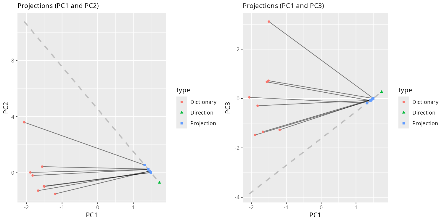
What cosine similarity is doing above, is measuring the distance between the projected point and the point corresponding to one pole of the semantic direction – in our case “huge.” The closer the projection is to that point, the more semantically similar it is to “huge.”
There is no technical restriction on what terms or concepts may be juxtaposed. So, you could define a direction away from “movies” toward “books,” but this direction may or may not organize the embedding space in a way that has face validity. As the paper shows (Grand et al. 2022), combinations of feature directions (e.g., wetness, danger) and objects (animals, cities) more highly correlated with human ratings than were others. Furthermore, with the semantic direction method discussed here, a built in assumption is that concepts can be adequately explained by a bipolar spectrum. This is an assumption which perhaps holds quite well for some things (like big to small) but not for others (like movies to books).