Concept Mover's Distance with Sensitivity Intervals
Source:vignettes/sensitivity-intervals-for-CMD.Rmd
sensitivity-intervals-for-CMD.Rmd
# pak::pkg_install(c("textclean", "gutenbergr", "stringi",
#                     "ggrepel", "tidyverse", "text2map"))
library(text2map)
library(tidyverse)

# optional
# pak::pkg_install("ggastrum")
if (requireNamespace("ggastrum", quietly = TRUE)) {
  ggastrum::set_theme()
}
Load some text data to work with:
data("meta_shakespeare")

# Grab the text from Project GUTENBERG
df_text <- meta_shakespeare |>
    select(gutenberg_id) |>
    gutenberg_download() |>
    group_by(gutenberg_id) |>
    summarize(text = paste(text, collapse = ", "))
Next, take care of a bit of preprocessing. Make sure there are no special characters, remove punctuation, take care of curly quotes (which can be a pain), and then squash contractions (rather than replacing apostrophes with a space, leaving a bunch of single letters). Finally, remove any digits that might be floating around. Then, make sure there is only a single space between and around words.
df_text <- df_text |> mutate(
    ## transliterate and lowercase
    text = stri_trans_general(text, id = "Any-Latin; Latin-ASCII"),
    text = tolower(text),
    ## punctuation
    text = replace_curly_quote(text),
    text = gsub("(\\w+[_'-]+\\w+)|[[:punct:]]+", "\\1", text),
    text = replace_contraction(text),
    ## remove numbers
    text = gsub('[[:digit:]]+', " ", text),
    ## take care of extra spaces
    text = gsub("[[:space:]]+", " ", text),
    text = trimws(text, whitespace = "[\\h\\v]")
)
Finally, we will need to convert the preprocessed text of the plays
into a Document-Term Matrix. The text2map package has a
very efficient unigram DTM builder called dtm_builder() –
it has very few options, but the unigram DTM is typically all we
need.
dtm <- df_text |>
       dtm_builder(text, gutenberg_id)
# text2map's handy DTM stats function
# let's just look at the basics
df_stats <- dtm_stats(dtm,
                    richness = FALSE,
                    distribution = FALSE,
                    central = FALSE,
                    character = FALSE
                    )

knitr::kable(df_stats, row.names = TRUE)| Measure | Value | |
|---|---|---|
| 1 | Total Docs | 37 |
| 2 | Percent Sparse | 87.70% |
| 3 | Total Types | 29957 |
| 4 | Total Tokens | 889429 |
| 5 | Object Size | 3.6 Mb |
Word Embeddings
You will need to load pre-trained word embeddings. We use the fastText
English embeddings. You can load it using
text2map.pretrained:
# install if necessary
remotes::install_gitlab("culturalcartography/text2map.pretrained")

library(text2map.pretrained)

# download once per machine
download_pretrained("vecs_fasttext300_wiki_news")

# load with data() once per session
data("vecs_fasttext300_wiki_news")
Concept Mover’s Distance
First, we will measure each play’s (defined by the DTM) closeness to
“death” using CMDist.
# Run CMD for concept words and semantic direction
cmd_plays <- dtm |>
    CMDist(cw = "death", # concept word
            wv = vecs_fasttext300_wiki_news, # word embeddings
            scale = FALSE)
Attach each CMD output to its respective play, using the gutenberg_id to join.
df <- cmd_plays |>
    rename(cmd_death = death) |>
    mutate(doc_id = as.numeric(doc_id) ) |>
    left_join(meta_shakespeare, by = c("doc_id" = "gutenberg_id")) |>
    as_tibble()
Let’s quickly plot closeness to “death” by a count of actual deaths in the play. This is roughly the same plot we included in our paper.
p_play <- df |>
   mutate(genre = as.factor(genre),
          shape = factor(boas_problem_plays,
                         levels = c(0, 1),
                         labels = c("", "Problem Play"))) |>
    ggplot(aes(x = body_count, y = cmd_death)) +
        geom_point(aes(color = genre, shape = shape), size = 3,  alpha = .9) +
        geom_text_repel(aes(label = short_title)) +
        scale_size(guide = "none") +
        labs(x = "Number of Deaths in the Play", y = "Closeness to 'Death'",
             title = NULL,
             color = "Genre",
             shape = "Boas' Problem Play",
             size = FALSE) +
        guides(shape = FALSE)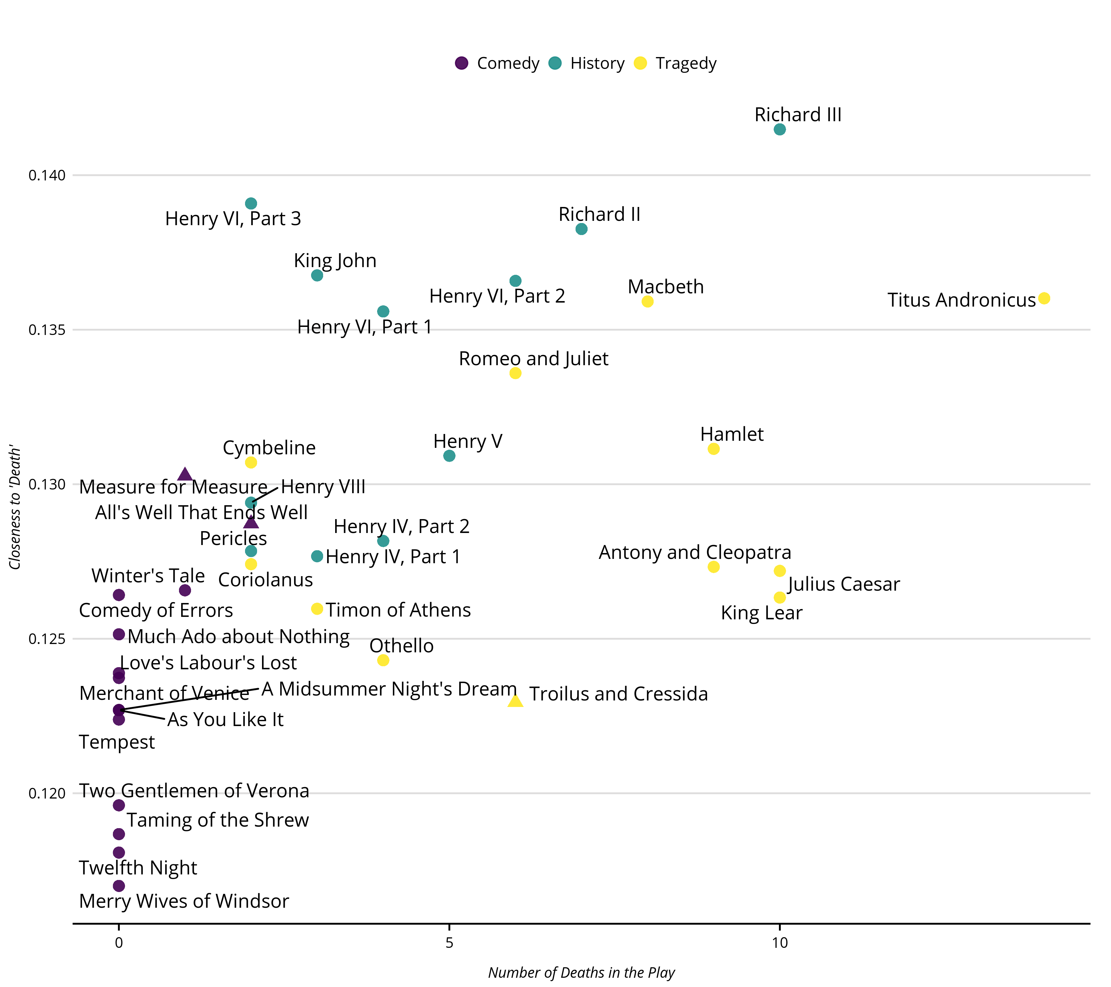
Sensitivity Intervals
If you recall, we did a little preprocessing at the beginning – and
typically analyst will do even more preprocessing. Recall, as
well, that in a DTM each document is represented as a distribution of
word counts. How “sensitive” is each estimate to a given distribution of
words? We can test this sensitivity by resampling (with replacement)
from each document’s word distribution. We do this by setting the
sens_interval=TRUES option in the CMDist()
function – underneath the hood, the CMDist() function is
using dtm_resampler() to estimate new DTMs and re-running
CMD on each, before reporting a given interval (default =
c(0.025, 0.975)). We will use the default settings for
now.
# Run CMD with sensitivity intervals
sens_plays <- CMDist(dtm = dtm,
cw = "death", # concept word
wv = vecs_fasttext300_wiki_news, # word embeddings
sens_interval = TRUE,
scale = TRUE)
df_sens <- sens_plays |>
rename(cmd_death = death) |>
mutate(doc_id = as.numeric(doc_id) ) |>
left_join(meta_shakespeare, by = c("doc_id" = "gutenberg_id")) |>
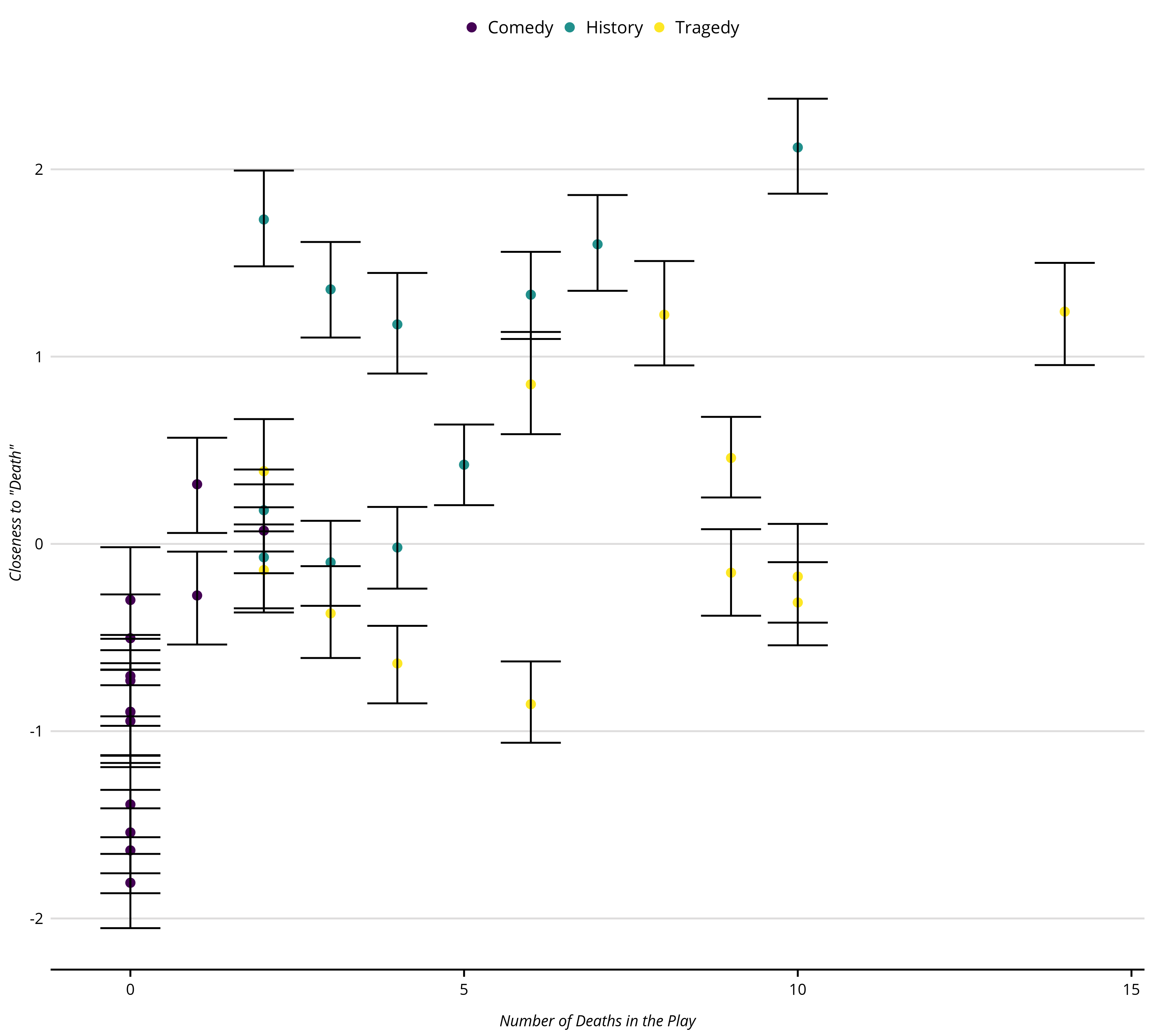
as_tibble()Now, we can plot the upper and lower bounds obtained from the resampled DTMs, along with the point estimate from the original DTM.
p_play_sens <- df_sens |>
    ggplot(aes(x = body_count, y = cmd_death)) +
    geom_point(aes(color = as.factor(genre)), size = 2) +
    geom_errorbar(aes(x = body_count, y = cmd_death,
                      ymin = death_lower,
                      ymax = death_upper),
                      color = "#000000") +
    xlab("Number of Deaths in the Play") +
    ylab('Closeness to "Death"')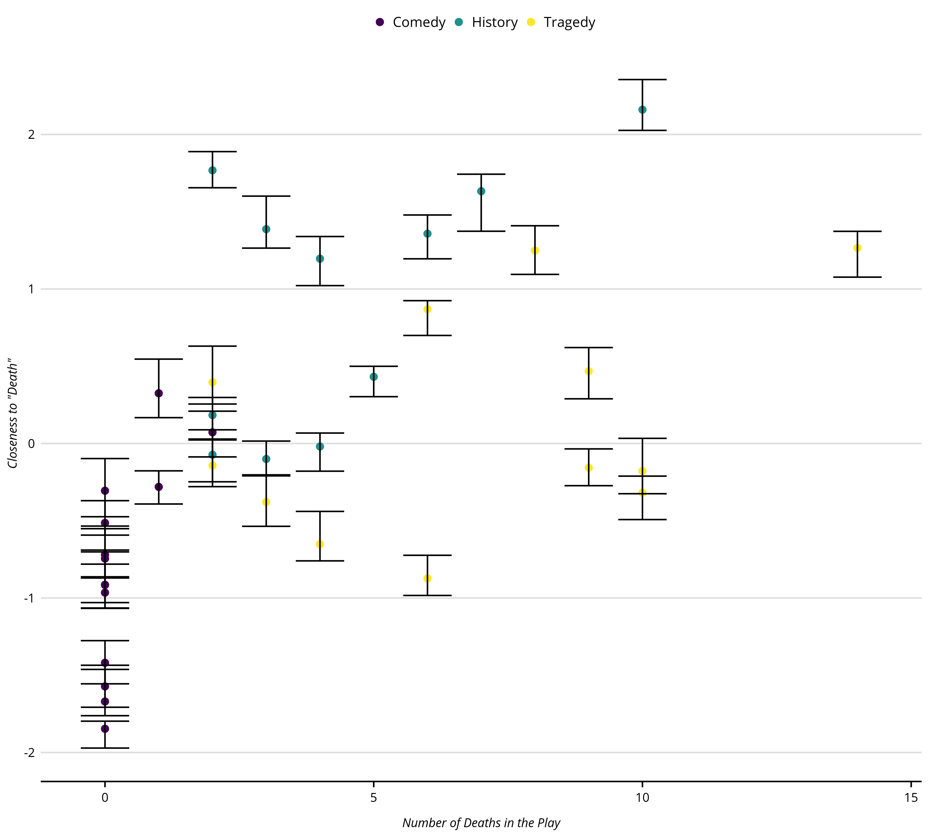
There are two optional parameters: alpha, and
n_iters. The first designates what proportion of the words
should be resampled. The default is 1, which means to resample the same
number of words as the original DTM row, whereas 0.5 would be to
resample half the number of words for each row, and 1.5 would be one and
half times more words than the original row. The default for
n_iters is the number of DTMs to resample. The default is
20.
# Run CMD with sensitivity intervals
play_sens_100 <- CMDist(
            dtm = dtm,
            cw = "death", # concept word
            wv = vecs_fasttext300_wiki_news, # word embeddings
            sens_interval = TRUE,
            alpha = 0.5,
            n_iters = 100L,
            scale = TRUE)

play_sens_100 <- play_sens_100L |>
    rename(cmd_death = death) |>
    mutate(doc_id = as.numeric(doc_id) ) |>
    left_join(meta_shakespeare, by = c("doc_id" = "gutenberg_id")) |>
    as_tibble()
Re-plot the estimates with sensitivity intervals from the new estimates using 100 resampled DTMs with rows half the size of the original DTM. Again, recall the point estimate are always from the original DTM – it is not an average across the sampled DTMs. Only the bounds are generated from the sampled DTMs.
p_play_sens_100 <- play_sens_100 |>
    ggplot(aes(x = body_count, y = death)) +
    geom_point(aes(color = as.factor(genre)), size = 2) +
    geom_errorbar(aes(x = body_count, y = death,
                      ymin = death_lower,
                      ymax = death_upper), color = "#000000") +
    xlab("Number of Deaths in the Play") +
    ylab('Closeness to "Death"')