Using Transformer-Based Contextual Embeddings with Concept Mover's Distance
Dustin S. Stoltz
2026-07-19
Source:vignettes/articles/using-transformers-contextual-BERT-with-CMD.Rmd
using-transformers-contextual-BERT-with-CMD.RmdContextual “Token” Embeddings
Static or word “type” embeddings create an embedding vector that aggregates all contexts into a single embedding vector for a given word type. In contrast, contextual or “token” embeddings – such as those based on Transformer models like ELMo, BERT, or DistilBERT – create an embedding vector for each token in a text.
Concept Mover’s Distance (Stoltz and Taylor 2019) or CMD is agnostic about the specific embeddings used, however, typically word “type” embeddings are used. How can contextual “token” embeddings be used with the method? There are actually two approaches:
- We could just use the token embeddings. The constraints of this approach primarily relate to the fact that the embeddings would be quite large – a vector for every token. We would still use relation induction techniques to derive a pseudo-document. For instance, if we are interested in the concept of death, we could average across all the individual death (and death-related) token vectors.
- We could average all the token embeddings into contextually-derived type embeddings. We then proceed exactly like a typical CMD analysis.
Below, we demonstrate how to take the second approach using
pretrained models hosted on Hugging Face and the text R package.
Preprocess Text
# pak::pkg_install(c("textclean", "gutenbergr", "stringi",
#                     "ggrepel", "tidyverse", "text2map", "text"))
library(text2map)
library(tidyverse)

# optional
# pak::pkg_install("ggastrum")
if (requireNamespace("ggastrum", quietly = TRUE)) {
  ggastrum::set_theme()
}
Load some text data to work with (you may need to find a different mirror):
data("meta_shakespeare")

my_mirror <- "https://mirror.csclub.uwaterloo.ca/gutenberg/"

# Grab the text from Project GUTENBERG
df_text <- meta_shakespeare |>
    select(gutenberg_id) |>
    gutenberg_download(mirror = my_mirror) |>
    group_by(gutenberg_id) |>
    summarise(text = paste(text, collapse = ", "))
Next, take care of a bit of preprocessing. Make sure there are no special characters, remove punctuation, take care of curly quotes (which can be a pain), and then squash contractions. Finally, remove any digits that might be floating around. Then, make sure there is only a single space between and around words.
df_text <- df_text |> mutate(
    ## transliterate and lowercase
    text = stri_trans_general(text, id = "Any-Latin; Latin-ASCII"),
    text = tolower(text),
    ## punctuation
    text = replace_curly_quote(text),
    text = gsub("(\\w+[_'-]+\\w+)|[[:punct:]]+", "\\1", text),
    text = replace_contraction(text),
    ## remove numbers
    text = gsub('[[:digit:]]+', " ", text),
    ## take care of extra spaces
    text = gsub("[[:space:]]+", " ", text),
    text = trimws(text, whitespace = "[\\h\\v]")
)
Fine-Tune the Contextual Embeddings
We will the distilBERT (Sanh et al. 2019), a smaller and snappier version of the base BERT model. We also lowercased our text, so we can use the uncased model. After training the embeddings, we’ll aggregate the token layers by averaging them to word types. This may take around 20 mins.
pretrained_model <- "distilbert-base-uncased"

embeddings <- textEmbed(
    text = df_text$text,
    model = pretrained_model,
    aggregation_from_tokens_to_word_types = "mean"
)
The embeddings object needs to be slightly reshaped:
Get Semantic Direction
Next we will want to create a “semantic direction” from are new
embedding space using the get_direction() function.
adds <- c("death")
subs <- c("life")
terms <- cbind(adds, subs)

sem_dir_dilbert <- get_direction(terms, wv_dilbert)
Using Concept Mover’s Distance
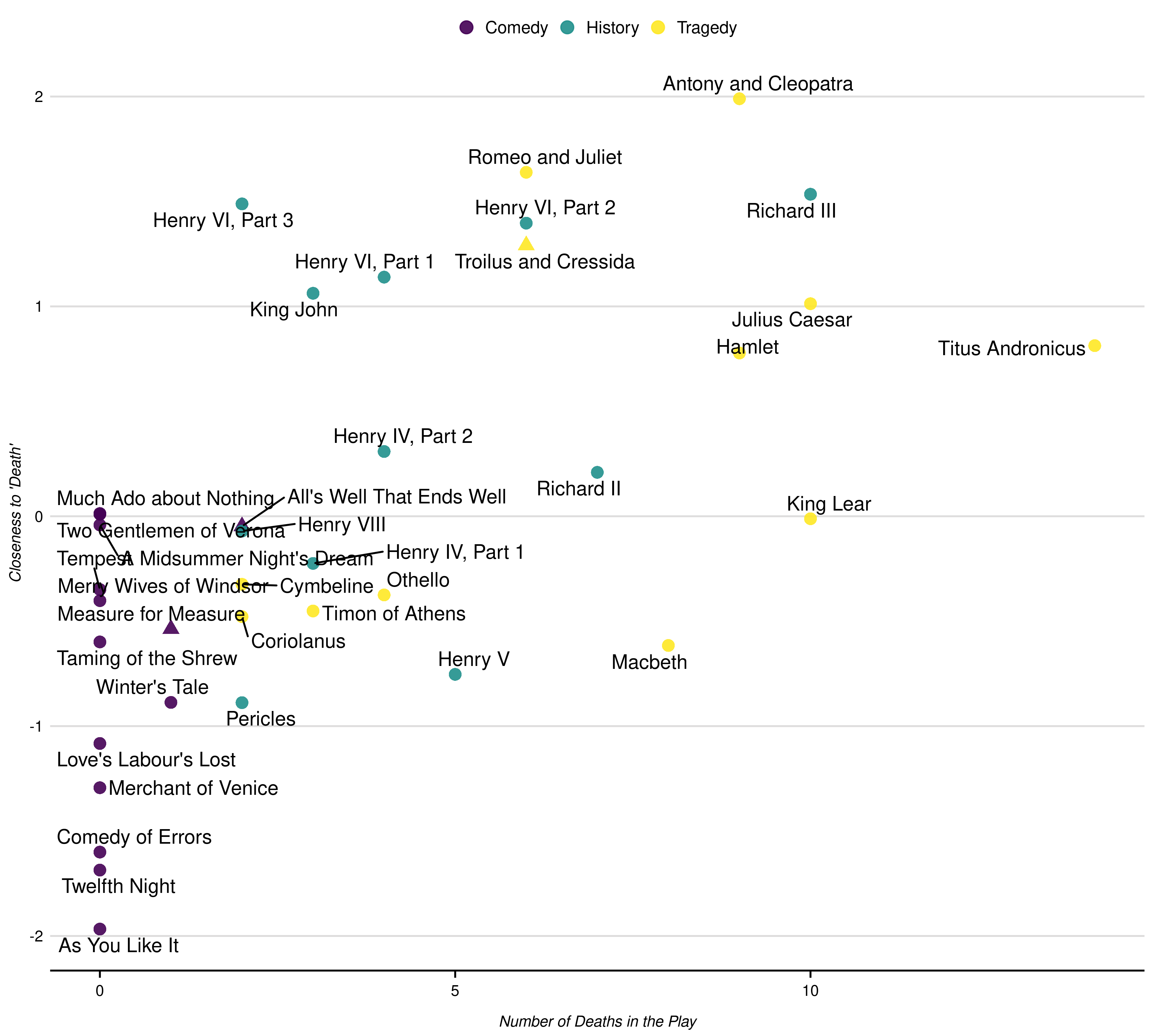
The next step is to use CMDist to measure how “close”
each of the words in the plays are to our semantic direction.
CMDist uses a DTM to represent the documents, and we will
use the terms in our embeddings (here, the row names) as the
“vocabulary” of our DTM, so they match exactly.
dtm_plays <- df_text |>
  dtm_builder(text = text,
              doc_id = gutenberg_id,
              vocab = rownames(wv_dilbert))
# Run CMD for concept words and semantic direction
cmd_plays <- dtm_plays |>
  CMDist(
    cv = sem_dir_dilbert,
    wv = wv_dilbert,
    scale = TRUE
  )

# combine with metadata
cmd_plays <- cmd_plays |>
  mutate(doc_id = as.numeric(doc_id)) |>
  left_join(meta_shakespeare,
    by = c("doc_id" = "gutenberg_id")
  ) |>
  rename(cmd_death = death_pole)
p_play <- cmd_plays |>
   mutate(genre = as.factor(genre),
          shape = factor(boas_problem_plays,
                         levels = c(0, 1),
                         labels = c("", "Problem Play"))) |>
    ggplot(aes(x = body_count, y = cmd_death)) +
        geom_point(aes(color = genre, shape = shape), size = 3,  alpha = .9) +
        geom_text_repel(aes(label = short_title)) +
        scale_size(guide = "none") +
        labs(x = "Number of Deaths in the Play", y = "Closeness to 'Death'",
             title = NULL,
             color = "Genre",
             shape = "Boas' Problem Play",
             size = FALSE) +
        guides(shape = FALSE)